Run a PyTorch binary classifier on CCI
Train a binary classifier on CCI with Jupyter + PyTorch — from environment setup to result visualization
Prerequisites
- You have an Alaya NeW enterprise account and password. If you need help or have not registered yet, follow Account setup to register.
- Your enterprise account has sufficient balance for using the Cloud Container Instance (CCI) service. Refer to the console for the latest promotion details and pricing.
This document walks you through running a complete machine learning project in Alaya NeW's Cloud Container Instance (CCI) using Jupyter Notebook. Even with zero prior experience, you can follow the steps and succeed!
🎯 Project goal
Train an AI model to distinguish between two classes of data points (just like teaching a child to tell apples from bananas), aiming for an accuracy above 90%.
🔧 Part 1: Environment preparation
Step 1: Enter Cloud Container Instance
- Log in to the console: Use your registered enterprise account to log in to the Alaya NeW platform. Click "Products > Compute > Cloud Container Instance" to enter the CCI page.
- Create a new cloud container: Click "New cloud container" to enter the CCI provisioning page, where you configure parameters such as instance name, instance description, and data center. For this example, configure each parameter as follows:
- Resource type: Select "Cloud Container Instance - GPU - H800A - 1 GPU".
- For other parameters, refer to the table below.
| Parameter | Description | Requirement | Required |
|---|---|---|---|
| Instance name | Identifier of the cloud container, used to uniquely identify it in the system | Must start with a letter; supports letters, digits, hyphens (-), and underscores (_); 4-20 characters | Yes |
| Instance description | A short text description of the cloud container's purpose, function, or configuration | None | No |
| Data center | The data center providing CCI service resources | Choose an available data center, e.g., Beijing Zone 3, Beijing Zone 5 | Yes |
| Billing mode | Billing method for using data center resources | Choose a supported billing mode (currently pay-as-you-go) | Yes |
| Resource configuration | Detailed resource specifications, including resource type, GPU model, compute spec, and disk configuration | Choose resources that meet your needs | Yes |
| Storage configuration | Optional NAS-type storage to mount into the CCI | Choose the NAS storage to mount | No |
| Image | Public images (base images and application images) and private images are supported. Choose the image type as needed | — | Yes |
| Other configuration | Configure environment-variable key-value pairs; optionally enable auto shutdown and auto release for the CCI | — | No |
-
Confirm provisioning: Once parameters are set, click "Provision now". In the confirmation dialog, verify the parameters and click "OK" to complete CCI provisioning.
You can check the created CCI on the Compute / Cloud Container Instance page. When the status shows "Running", the instance is ready to use.
-
Open Jupyter: Click the access URL to enter the Jupyter UI.

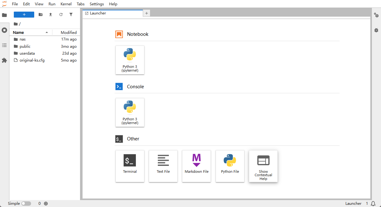
- Jupyter home: You will see the screen below.
Step 2: Open a terminal
In the "Launcher" area on the right side of the Jupyter UI:
- Under "Other", click "Terminal".
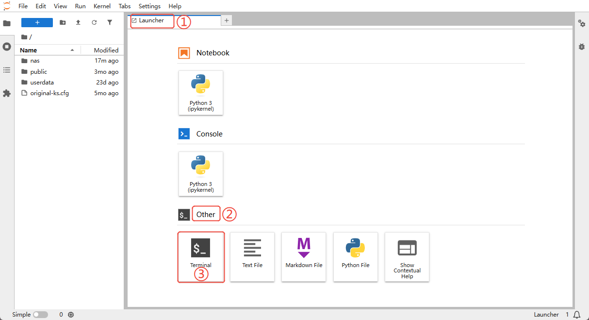
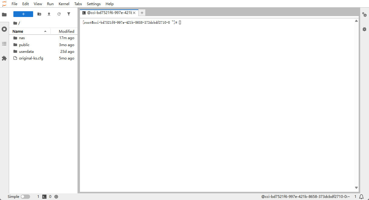
- A command-line window opens.
Step 3: Install required packages
This document uses Ubuntu as the example OS.
# Install venv
apt update && apt install python3.12-venv -y

# Remove the old virtual environment (if any)
rm -rf ml_env

# Create a new virtual environment
python3 -m venv ml_env

# Activate the environment
source ml_env/bin/activate

# Install packages
pip install --upgrade pip
pip install numpy matplotlib torch torchvision jupyter ipykernel

# Register the Jupyter kernel
python -m ipykernel install --user --name=ml_env --display-name="Python (ml_env)"

# Verify
echo "Environment setup complete!"
python -c "import numpy; print('NumPy version:', numpy.__version__)"
python -c "import torch; print('PyTorch version:', torch.__version__)"

echo "Refresh the Jupyter page, then choose the 'Python (ml_env)' kernel when creating a Notebook"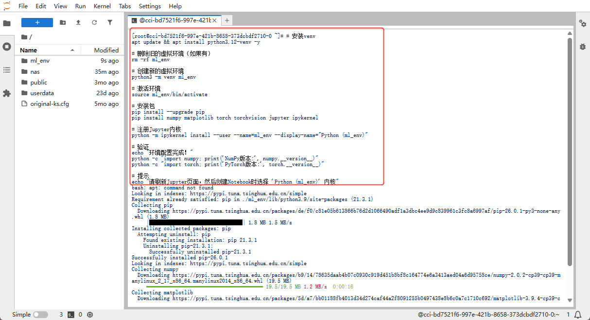
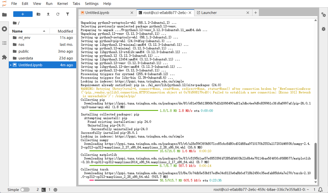
Installation in progress 👇
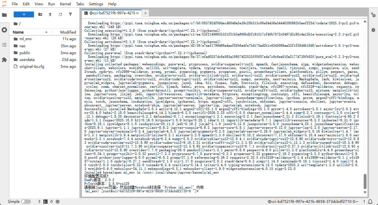
Installation complete 👇
Check the system version
If you are unsure about your OS version, run the following commands in the terminal to inspect system info:
# Method 1: View the OS release file
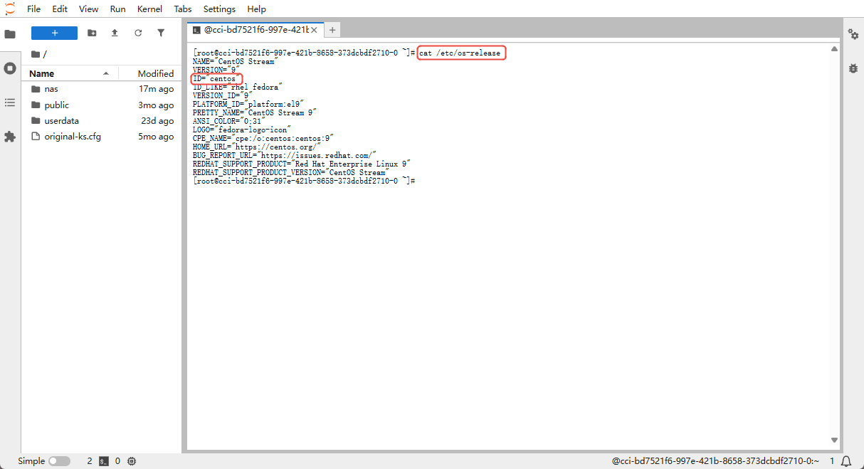
cat /etc/os-release
# Method 2: Print system info
uname -a
# Method 3: View Linux release info
cat /etc/*release*You will see output similar to the following:
- Ubuntu / Debian: shows
ID=ubuntuorID=debian - CentOS / RHEL: shows
ID="centos"orID="rhel" - Alpine: shows
ID=alpine
Install commands differ across operating systems.
Step 4: Verify the installation
Continue in the terminal:
# Check NumPy installation
python -c "import numpy; print('NumPy version:', numpy.__version__)"

# Check PyTorch installation
python -c "import torch; print('PyTorch version:', torch.__version__)"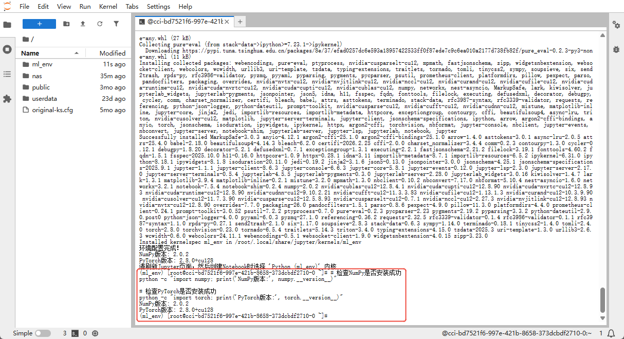
📝 Part 2: Create and run the machine learning code
Step 1: Refresh the Jupyter page
Refresh your browser so the newly installed environment takes effect.
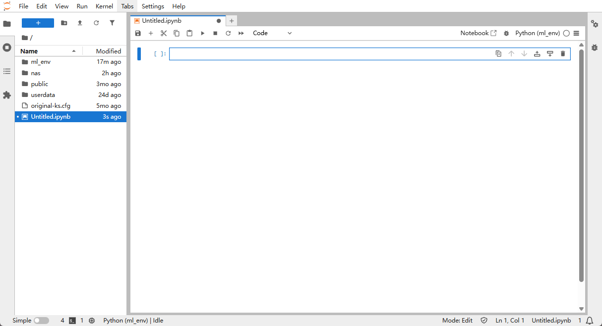
Step 2: Create a new Notebook
- Close the Terminal window and return to the Launcher page. The UI looks like the screenshot below.
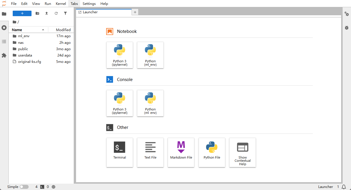
- In the Notebook section, locate "Python (ml_env)" (the environment we just created) and click it.

Step 3: Paste in the code
Copy the code below into your Notebook in chunks. We recommend using 6 cells for easier reading and debugging.
Cell 1: Import the required libraries
Copy the code below into a cell and press Shift + Enter to run it.
import math
import time
import random
import numpy as np
import matplotlib.pyplot as plt
import torch
import torch.nn as nn
from torch.utils.data import TensorDataset, DataLoader
from pathlib import Path
# Set random seeds (for reproducible results across runs)
def set_seed(seed=42):
random.seed(seed)
np.random.seed(seed)
torch.manual_seed(seed)
if torch.cuda.is_available():
torch.cuda.manual_seed_all(seed)
torch.backends.cudnn.deterministic = True
set_seed(42)
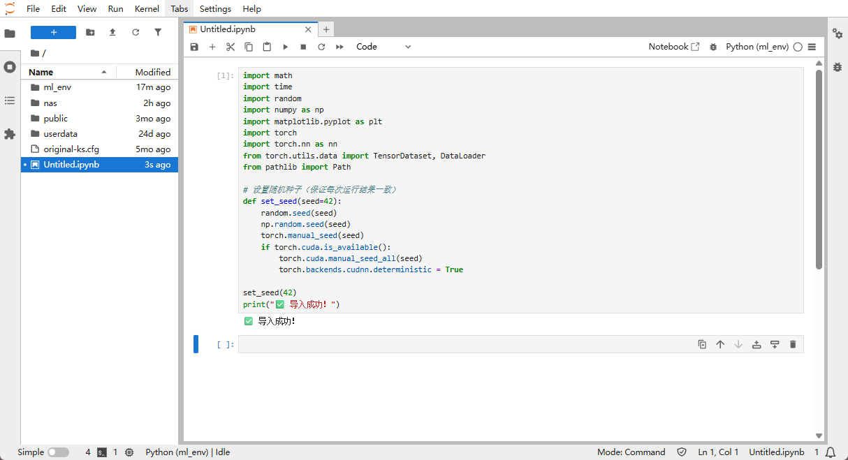
print("✅ Imports successful!")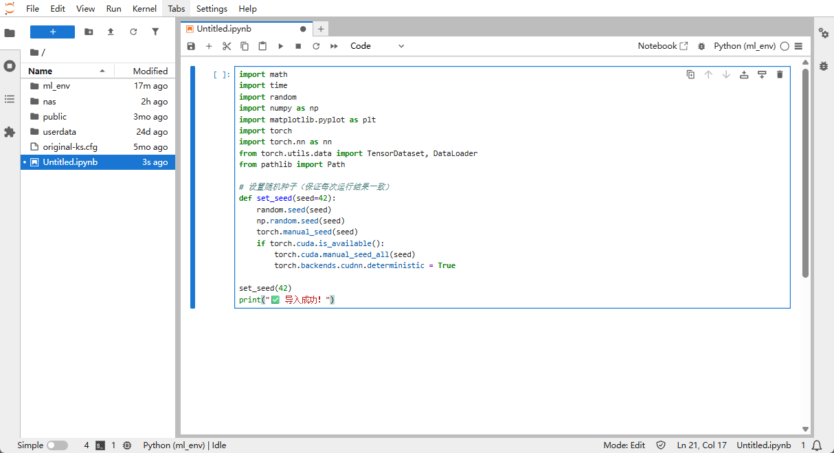
Successful output 👇
Cell 2: Build the dataset
Copy the code below into a cell and press Shift + Enter to run it.
def make_moons(n_samples=1000, noise=0.2):
    """Generate a two-moons dataset"""
    n_samples_out = n_samples // 2
    n_samples_in = n_samples - n_samples_out
    outer_circ_x = np.cos(np.linspace(0, math.pi, n_samples_out))
    outer_circ_y = np.sin(np.linspace(0, math.pi, n_samples_out))
    inner_circ_x = 1 - np.cos(np.linspace(0, math.pi, n_samples_in))
    inner_circ_y = 1 - np.sin(np.linspace(0, math.pi, n_samples_in)) - .5
    X = np.vstack([np.append(outer_circ_x, inner_circ_x),
                    np.append(outer_circ_y, inner_circ_y)]).T.astype(np.float32)
    y = np.hstack([np.zeros(n_samples_out, dtype=np.float32),
                    np.ones(n_samples_in,  dtype=np.float32)])
    if noise > 0:
        X += np.random.normal(0, noise, X.shape)
    return X, y

# Build a dataset of 1200 samples
X, y = make_moons(1200, noise=0.25)

# Split into training (80%) and validation (20%) sets
perm = np.random.permutation(len(X))
train_size = int(0.8 * len(X))
X_train, y_train = X[perm[:train_size]], y[perm[:train_size]]
X_val, y_val = X[perm[train_size:]], y[perm[train_size:]]

# Build the data loaders (for mini-batch training)
train_ds = TensorDataset(torch.from_numpy(X_train), torch.from_numpy(y_train))
val_ds = TensorDataset(torch.from_numpy(X_val), torch.from_numpy(y_val))
train_loader = DataLoader(train_ds, batch_size=64, shuffle=True)
val_loader = DataLoader(val_ds, batch_size=256, shuffle=False)

print(f"Training samples: {len(train_ds)}")
print(f"Validation samples: {len(val_ds)}")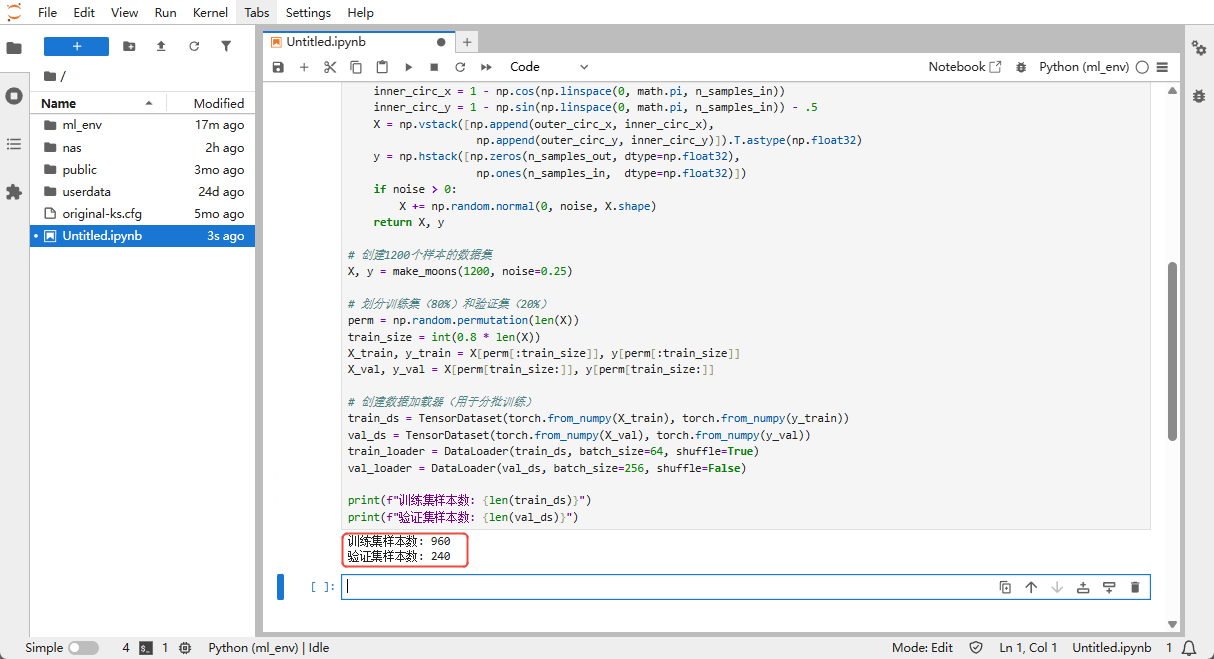
Cell 3: Define the neural network model
Copy the code below into a cell and press Shift + Enter to run it.
class MLP(nn.Module):
"""A simple neural network"""
def __init__(self, in_dim=2, hidden=128, dropout_rate=0.2):
super().__init__()
self.net = nn.Sequential(
nn.Linear(in_dim, hidden), # Input layer → hidden layer 1
nn.ReLU(), # Activation function
nn.Dropout(dropout_rate), # Prevent overfitting
nn.Linear(hidden, hidden//2), # Hidden layer 1 → hidden layer 2
nn.ReLU(),
nn.Dropout(dropout_rate),
nn.Linear(hidden//2, 1) # Hidden layer 2 → output layer
)
def forward(self, x):
return self.net(x).squeeze(1)
# Check whether a GPU is available
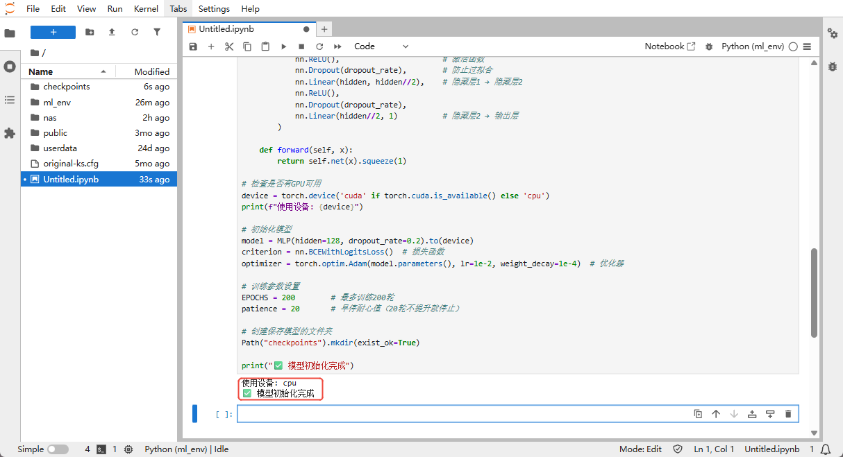
device = torch.device('cuda' if torch.cuda.is_available() else 'cpu')
print(f"Using device: {device}")
# Initialize the model
model = MLP(hidden=128, dropout_rate=0.2).to(device)
criterion = nn.BCEWithLogitsLoss() # Loss function
optimizer = torch.optim.Adam(model.parameters(), lr=1e-2, weight_decay=1e-4) # Optimizer
# Training hyperparameters
EPOCHS = 200 # Train for at most 200 epochs
patience = 20 # Early-stopping patience (stop if no improvement for 20 epochs)
# Create a folder to save model checkpoints
Path("checkpoints").mkdir(exist_ok=True)
print("✅ Model initialized")
Cell 4: Define helper functions
Copy the code below into a cell and press Shift + Enter to run it.
# Set up live plotting
plt.ion()
fig = plt.figure(figsize=(15, 6))
ax_loss = fig.add_subplot(1, 2, 1) # Left: loss curves
ax_boundary = fig.add_subplot(1, 2, 2) # Right: decision boundary
train_losses, val_losses = [], [] # Track losses
train_accs, val_accs = [], [] # Track accuracy
def calculate_accuracy(model, data_loader):
"""Compute the model's accuracy"""
model.eval()
correct = 0
total = 0
with torch.no_grad():
for xb, yb in data_loader:
xb, yb = xb.to(device), yb.to(device)
outputs = torch.sigmoid(model(xb))
predicted = (outputs > 0.5).float()
total += yb.size(0)
correct += (predicted == yb).sum().item()
return correct / total
def plot_boundary(ax, epoch):
"""Plot the decision boundary"""
ax.clear()
h = 0.02
x_min, x_max = X[:, 0].min() - .5, X[:, 0].max() + .5
y_min, y_max = X[:, 1].min() - .5, X[:, 1].max() + .5
xx, yy = np.meshgrid(np.arange(x_min, x_max, h),
np.arange(y_min, y_max, h))
grid = torch.from_numpy(np.c_[xx.ravel(), yy.ravel()]).float().to(device)
with torch.no_grad():
Z = torch.sigmoid(model(grid)).cpu().numpy().reshape(xx.shape)
ax.contourf(xx, yy, Z, levels=50, cmap='RdBu', alpha=0.7)
ax.scatter(X_train[:, 0], X_train[:, 1], c=y_train, cmap='bwr',
edgecolors='k', marker='o', label='Training set', alpha=0.7)
ax.scatter(X_val[:, 0], X_val[:, 1], c=y_val, cmap='bwr',
edgecolors='k', marker='x', label='Validation set', alpha=0.7)
ax.set_xlim(xx.min(), xx.max())
ax.set_ylim(yy.min(), yy.max())
ax.set_title(f'Decision boundary (epoch {epoch})')
ax.legend()
def plot_metrics(ax):
"""Plot loss and accuracy curves"""
ax.clear()
ax.plot(train_losses, label='Training loss', color='blue', linestyle='-')
ax.plot(val_losses, label='Validation loss', color='red', linestyle='-')
ax.set_xlabel('Epoch')
ax.set_ylabel('Loss', color='black')
ax.legend(loc='upper left')
ax.grid(True)
ax2 = ax.twinx()
ax2.plot(train_accs, label='Training accuracy', color='blue', linestyle='--')
ax2.plot(val_accs, label='Validation accuracy', color='red', linestyle='--')
ax2.set_ylabel('Accuracy', color='black')
ax2.legend(loc='upper right')
ax.set_title('Training progress')
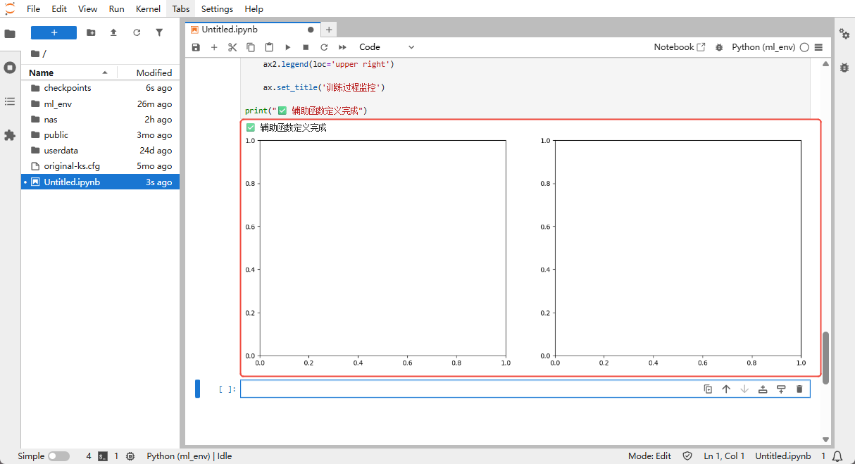
print("✅ Helper functions defined")
Cell 5: Run training (the core)
Copy the code below into a cell and press Shift + Enter to run it.
print("🚀 Starting training...")
start_time = time.time()
best_val_loss = float('inf')
patience_counter = 0
for epoch in range(1, EPOCHS + 1):
# ----- Training phase -----
model.train()
epoch_loss = 0.
for xb, yb in train_loader:
xb, yb = xb.to(device), yb.to(device)
optimizer.zero_grad()
logits = model(xb)
loss = criterion(logits, yb)
loss.backward()
optimizer.step()
epoch_loss += loss.item() * xb.size(0)
train_loss = epoch_loss / len(train_loader.dataset)
train_losses.append(train_loss)
# ----- Validation phase -----
model.eval()
epoch_loss = 0.
with torch.no_grad():
for xb, yb in val_loader:
xb, yb = xb.to(device), yb.to(device)
logits = model(xb)
loss = criterion(logits, yb)
epoch_loss += loss.item() * xb.size(0)
val_loss = epoch_loss / len(val_loader.dataset)
val_losses.append(val_loss)
# Compute accuracy
train_acc = calculate_accuracy(model, train_loader)
val_acc = calculate_accuracy(model, val_loader)
train_accs.append(train_acc)
val_accs.append(val_acc)
# Print progress every 10 epochs
if epoch % 10 == 0 or epoch == 1:
print(f'Epoch {epoch:03d}/200 | '
f'Train loss: {train_loss:.4f} | Val loss: {val_loss:.4f} | '
f'Train acc: {train_acc:.3f} | Val acc: {val_acc:.3f}')
# Save the best model
if val_loss < best_val_loss:
best_val_loss = val_loss
patience_counter = 0
torch.save({
'epoch': epoch,
'model_state_dict': model.state_dict(),
'loss': val_loss,
}, 'checkpoints/best_model.pth')
else:
patience_counter += 1
# Early stopping (stop if no improvement for 20 epochs)
if patience_counter >= patience:
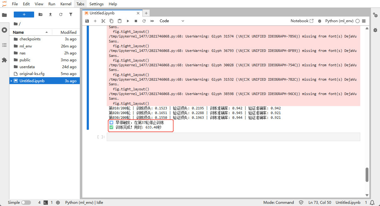
print(f"⏹️ Early stopping triggered at epoch {epoch}")
break
# Refresh the plots every 5 epochs
if epoch % 5 == 0 or epoch == 1:
plot_metrics(ax_loss)
plot_boundary(ax_boundary, epoch)
fig.tight_layout()
plt.pause(0.01)
end_time = time.time()
print(f"✅ Training complete! Elapsed: {end_time - start_time:.2f}s")

Cell 6: Final evaluation and visualization
Copy the code below into a cell and press Shift + Enter to run it.
# Load the best model
checkpoint = torch.load('checkpoints/best_model.pth')
model.load_state_dict(checkpoint['model_state_dict'])
print(f"📥 Loaded best model (epoch {checkpoint['epoch']}, val loss: {checkpoint['loss']:.4f})")
# Final evaluation
model.eval()
with torch.no_grad():
X_tensor = torch.from_numpy(X).to(device)
y_pred_proba = torch.sigmoid(model(X_tensor)).cpu().numpy()
y_pred = (y_pred_proba > 0.5).astype(int)
accuracy = (y_pred == y).mean()
print(f'🎯 Final accuracy: {accuracy:.3f} ({accuracy*100:.1f}%)')
# Render the final plots
plt.figure(figsize=(15, 6))
# Left: loss and accuracy curves
plt.subplot(1, 2, 1)
plt.plot(train_losses, label='Training loss', color='blue', linestyle='-')
plt.plot(val_losses, label='Validation loss', color='red', linestyle='-')
plt.xlabel('Epoch')
plt.ylabel('Loss')
plt.legend(loc='upper left')
plt.twinx()
plt.plot(train_accs, label='Training accuracy', color='blue', linestyle='--')
plt.plot(val_accs, label='Validation accuracy', color='red', linestyle='--')
plt.ylabel('Accuracy')
plt.legend(loc='upper right')
plt.title('Training progress')
plt.grid(True)
# Right: decision boundary
plt.subplot(1, 2, 2)
h = 0.02
x_min, x_max = X[:, 0].min() - .5, X[:, 0].max() + .5
y_min, y_max = X[:, 1].min() - .5, X[:, 1].max() + .5
xx, yy = np.meshgrid(np.arange(x_min, x_max, h),
np.arange(y_min, y_max, h))
grid = torch.from_numpy(np.c_[xx.ravel(), yy.ravel()]).float().to(device)
with torch.no_grad():
Z = torch.sigmoid(model(grid)).cpu().numpy().reshape(xx.shape)
plt.contourf(xx, yy, Z, levels=50, cmap='RdBu', alpha=0.7)
plt.scatter(X_train[:, 0], X_train[:, 1], c=y_train, cmap='bwr',
edgecolors='k', marker='o', label='Training set', alpha=0.7)
plt.scatter(X_val[:, 0], X_val[:, 1], c=y_val, cmap='bwr',
edgecolors='k', marker='x', label='Validation set', alpha=0.7)
plt.colorbar()
plt.xlim(xx.min(), xx.max())
plt.ylim(yy.min(), yy.max())
plt.title('Final decision boundary')
plt.legend()
plt.tight_layout()
plt.show()
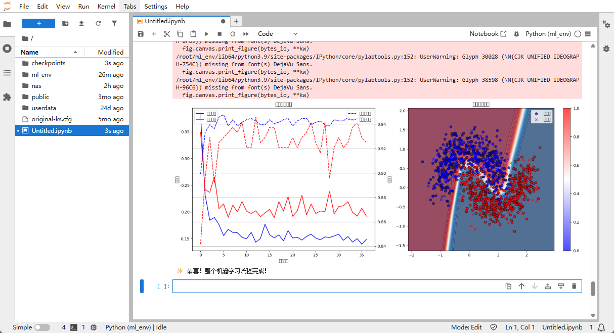
print("✨ Congratulations! The full machine learning workflow is complete!")
📊 Part 3: Interpreting the results
Reading the training output
Epoch 001/200 | Train loss: 0.3820 | Val loss: 0.3491 | Train acc: 0.899 | Val acc: 0.842
Epoch 010/200 | Train loss: 0.1523 | Val loss: 0.2195 | Train acc: 0.942 | Val acc: 0.942- Loss: lower is better; indicates fewer prediction errors.
- Accuracy: higher is better; the fraction of correct predictions.
- Final accuracy: e.g., 0.942 means 94.2% accuracy.
Reading the plots
- Left plot: blue line = training set, red line = validation set
- Solid lines are loss values (lower is better)
- Dashed lines are accuracy values (higher is better)
- Right plot:
- Colored background: the model's predicted regions
- Red/blue points: ground-truth data (circles = training set, crosses = validation set)
🎉 Summary
In this exercise you have:
- ✅ Configured a Python environment in a cloud container
- ✅ Built a neural network model
- ✅ Trained the model to distinguish two classes of data
- ✅ Reached over 90% accuracy
- ✅ Visualized the model's decision process
This is just like teaching an AI "kid" to recognize two kinds of objects — once trained, it can classify new ones. The core of machine learning is the loop: "feed data → let the model learn → use the model to predict".
Last updated on
Run a LoRA fine-tune with LLaMA Factory on CCI
Install LLaMA Factory in a CCI instance and run a LoRA SFT pass via the WebUI (Llama-3-8B-Instruct as the example)
Deploy an OpenAI-compatible inference service with vLLM on CCI
Install vLLM in a CCI instance, download the model, launch an OpenAI-compatible inference server, and verify with curl