Machine Learning on Cloud Container Instances

Updated at: 2025-12-01 17:01:25

This section describes how to perform machine learning on Cloud Container Instances.

Prerequisites

You have obtained your Alaya NeW company account and password. If you need assistance or have not registered yet, you can complete the registration by following the instructions in User Registration.
Your company account has sufficient balance to use the Cloud Container Instance service. For the latest promotional details and pricing information, please Contact US.

Procedure

Step 1: Create a Cloud Container Instance

Sign in to the Alaya NeW platform using your company account. Choose "Product" > "Computing" > "Cloud Container Instance" to enter the CCI page.

Choose [Create Cloud Container Instance] to open the instance creation page. Configure the instance name, description, AIDC, and other parameters.

In this example, configure the parameters as follows:

Resource Type: Select "Cloud Container Instance – GPU H800A (1 GPU)".

For other parameters, refer to the table below.

Configuration Item	Description	Requirements	Required
Instance Name	A unique identifier used to distinguish this Cloud Container Instance.	Must start with a letter; supports letters, digits, hyphens (-), and underscores (_); length 4–20 characters.	Yes
Instance Description	A brief text description of the container’s purpose, usage, or configuration.	None	No
AIDC	The data center used to support cloud container instance service.	Select an available data center (for example, Beijing Region 3 or Beijing Region 5).	Yes
Payment Method	The method for using data center resources.	Select the supported payment method. Currently, Pay-As-You-Go is used.	Yes
Resource Configuration	Detailed compute resource specifications, including resource type, GPU, compute resource, and disk configuration.	Select resources that meet your requirements.	Yes
Storage Configuration	Optional NAS storage that can be mounted to the Cloud Container Instance	Choose whether to mount NAS storage.	No
Image	You can choose from public images (including base images and application images) or private images, depending on your needs.	-	Yes
Other Settings	Supports configuring environment variables (key–value pairs), and enabling auto-shutdown and auto-release for the Cloud Container Instance.	-	No

After configuring the instance parameters, choose "Create Now". In the confirmation dialog box, review the configured parameters and choose "Confirm" to complete the creation of the Cloud Container Instance.

You can view the created instances on the [Computing / Cloud Container Instance] page. When the instance status is "Running", the instance has been created successfully and is ready for use.

Step 2: Perform Machine Learning Tasks

Enter Jupyter.

On the "Cloud Container Instance" page, open the "Container List" tab and locate the target instance. Choose the Jupyter icon on the right to open the Jupyter environment.

Execute the following to build a machine learning training workflow.

Code details

import math
import time
import random
import numpy as np
import matplotlib.pyplot as plt
import torch
import torch.nn as nn
from torch.utils.data import TensorDataset, DataLoader
from pathlib import Path

# Set random seeds to ensure reproducibility
def set_seed(seed=42):
    random.seed(seed)
    np.random.seed(seed)
    torch.manual_seed(seed)
    if torch.cuda.is_available():
        torch.cuda.manual_seed_all(seed)
        torch.backends.cudnn.deterministic = True

set_seed(42)

def make_moons(n_samples=1000, noise=0.2):
    """Implement make_moons manually without relying on sklearn"""
    n_samples_out = n_samples // 2
    n_samples_in = n_samples - n_samples_out
    outer_circ_x = np.cos(np.linspace(0, math.pi, n_samples_out))
    outer_circ_y = np.sin(np.linspace(0, math.pi, n_samples_out))
    inner_circ_x = 1 - np.cos(np.linspace(0, math.pi, n_samples_in))
    inner_circ_y = 1 - np.sin(np.linspace(0, math.pi, n_samples_in)) - .5
    X = np.vstack([np.append(outer_circ_x, inner_circ_x),
                    np.append(outer_circ_y, inner_circ_y)]).T.astype(np.float32)
    y = np.hstack([np.zeros(n_samples_out, dtype=np.float32),
                    np.ones(n_samples_in,  dtype=np.float32)])
    if noise > 0:
        X += np.random.normal(0, noise, X.shape)
    return X, y

# Create dataset
X, y = make_moons(1200, noise=0.25)

# Split into training and validation sets
perm = np.random.permutation(len(X))
train_size = int(0.8 * len(X))
X_train, y_train = X[perm[:train_size]], y[perm[:train_size]]
X_val, y_val = X[perm[train_size:]], y[perm[train_size:]]

# Create data loaders
train_ds = TensorDataset(torch.from_numpy(X_train), torch.from_numpy(y_train))
val_ds = TensorDataset(torch.from_numpy(X_val), torch.from_numpy(y_val))
train_loader = DataLoader(train_ds, batch_size=64, shuffle=True)
val_loader = DataLoader(val_ds, batch_size=256, shuffle=False)

class MLP(nn.Module):
    def __init__(self, in_dim=2, hidden=128, dropout_rate=0.2):
        super().__init__()
        self.net = nn.Sequential(
            nn.Linear(in_dim, hidden),
            nn.ReLU(),
            nn.Dropout(dropout_rate),
            nn.Linear(hidden, hidden//2),
            nn.ReLU(),
            nn.Dropout(dropout_rate),
            nn.Linear(hidden//2, 1)
        )
        
    def forward(self, x):
        return self.net(x).squeeze(1)

# Set device
device = torch.device('cuda' if torch.cuda.is_available() else 'cpu')
print(f"Using device: {device}")

# Initialize model, loss, and optimizer
model = MLP(hidden=128, dropout_rate=0.2).to(device)
criterion = nn.BCEWithLogitsLoss()
optimizer = torch.optim.Adam(model.parameters(), lr=1e-2, weight_decay=1e-4)
scheduler = torch.optim.lr_scheduler.ReduceLROnPlateau(
    optimizer, mode='min', factor=0.5, patience=10
)

# Training parameters
EPOCHS = 200
PLOT_FREQ = 5  # Plot the graph every 5 epochs
best_val_loss = float('inf')
patience_counter = 0
patience = 20  # early stopping patience

# Create directory for saving models
Path("checkpoints").mkdir(exist_ok=True)

# Enable interactive plotting
plt.ion()
fig = plt.figure(figsize=(15, 6))
ax_loss = fig.add_subplot(1, 2, 1)
ax_boundary = fig.add_subplot(1, 2, 2)

train_losses, val_losses = [], []
train_accs, val_accs = [], []

def calculate_accuracy(model, data_loader):
    """Calculate model accuracy on the given DataLoader"""
    model.eval()
    correct = 0
    total = 0
    with torch.no_grad():
        for xb, yb in data_loader:
            xb, yb = xb.to(device), yb.to(device)
            outputs = torch.sigmoid(model(xb))
            predicted = (outputs > 0.5).float()
            total += yb.size(0)
            correct += (predicted == yb).sum().item()
    return correct / total

def plot_boundary(ax, epoch):
    """Plot decision boundary"""
    ax.clear()
    # Create grid
    h = 0.02
    x_min, x_max = X[:, 0].min() - .5, X[:, 0].max() + .5
    y_min, y_max = X[:, 1].min() - .5, X[:, 1].max() + .5
    xx, yy = np.meshgrid(np.arange(x_min, x_max, h),
                            np.arange(y_min, y_max, h))
    
    # Predict grid points
    grid = torch.from_numpy(np.c_[xx.ravel(), yy.ravel()]).float().to(device)
    with torch.no_grad():
        Z = torch.sigmoid(model(grid)).cpu().numpy().reshape(xx.shape)
    
    # Draw decision boundary
    contour = ax.contourf(xx, yy, Z, levels=50, cmap='RdBu', alpha=0.7)
    
    # Plot data points
    ax.scatter(X_train[:, 0], X_train[:, 1], c=y_train, cmap='bwr', 
                edgecolors='k', marker='o', label='Train', alpha=0.7)
    ax.scatter(X_val[:, 0], X_val[:, 1], c=y_val, cmap='bwr', 
                edgecolors='k', marker='x', label='Val', alpha=0.7)
    
    ax.set_xlim(xx.min(), xx.max())
    ax.set_ylim(yy.min(), yy.max())
    ax.set_title(f'Decision Boundary (Epoch {epoch})')
    ax.legend()
    plt.colorbar(contour, ax=ax)

def plot_metrics(ax):
    """Plot loss and accuracy curves"""
    ax.clear()
    
    # Plot losses
    ax.plot(train_losses, label='Train Loss', color='blue', linestyle='-')
    ax.plot(val_losses, label='Val Loss', color='red', linestyle='-')
    ax.set_xlabel('Epoch')
    ax.set_ylabel('Loss', color='black')
    ax.tick_params(axis='y', labelcolor='black')
    ax.legend(loc='upper left')
    
    # Create second y-axis for accuracy
    ax2 = ax.twinx()
    ax2.plot(train_accs, label='Train Acc', color='blue', linestyle='--')
    ax2.plot(val_accs, label='Val Acc', color='red', linestyle='--')
    ax2.set_ylabel('Accuracy', color='black')
    ax2.tick_params(axis='y', labelcolor='black')
    ax2.legend(loc='upper right')
    
    ax.set_title('Training Metrics')
    ax.grid(True)

# Training loop
start_time = time.time()
for epoch in range(1, EPOCHS + 1):
    # Training phase
    model.train()
    epoch_loss = 0.
    for xb, yb in train_loader:
        xb, yb = xb.to(device), yb.to(device)
        optimizer.zero_grad()
        logits = model(xb)
        loss = criterion(logits, yb)
        loss.backward()
        optimizer.step()
        epoch_loss += loss.item() * xb.size(0)
    
    train_loss = epoch_loss / len(train_loader.dataset)
    train_losses.append(train_loss)
    
    # Validation phase
    model.eval()
    epoch_loss = 0.
    with torch.no_grad():
        for xb, yb in val_loader:
            xb, yb = xb.to(device), yb.to(device)
            logits = model(xb)
            loss = criterion(logits, yb)
            epoch_loss += loss.item() * xb.size(0)
    
    val_loss = epoch_loss / len(val_loader.dataset)
    val_losses.append(val_loss)
    
    # Calculate accuracy
    train_acc = calculate_accuracy(model, train_loader)
    val_acc = calculate_accuracy(model, val_loader)
    train_accs.append(train_acc)
    val_accs.append(val_acc)
    
    # Scheduler step
    scheduler.step(val_loss)
    
    # Print progress
    if epoch % 10 == 0 or epoch == 1:
        print(f'Epoch {epoch:03d}/{EPOCHS} | '
                f'Train Loss: {train_loss:.4f} | Val Loss: {val_loss:.4f} | '
                f'Train Acc: {train_acc:.3f} | Val Acc: {val_acc:.3f} | '
                f'LR: {optimizer.param_groups[0]["lr"]:.2e}')
    
    # Save best model
    if val_loss < best_val_loss:
        best_val_loss = val_loss
        patience_counter = 0
        torch.save({
            'epoch': epoch,
            'model_state_dict': model.state_dict(),
            'optimizer_state_dict': optimizer.state_dict(),
            'loss': val_loss,
        }, 'checkpoints/best_model.pth')
    else:
        patience_counter += 1
    
    # Early stopping check
    if patience_counter >= patience:
        print(f"Early stopping at epoch {epoch}")
        break
    
    # Visualization
    if epoch % PLOT_FREQ == 0 or epoch == 1 or epoch == EPOCHS:
        plot_metrics(ax_loss)
        plot_boundary(ax_boundary, epoch)
        fig.tight_layout()
        plt.pause(0.01)

# Training finished
end_time = time.time()
print(f"Training completed in {end_time - start_time:.2f} seconds")

# Turn off interactive mode
plt.ioff()

# Load best model
checkpoint = torch.load('checkpoints/best_model.pth')
model.load_state_dict(checkpoint['model_state_dict'])
print(f"Loaded best model from epoch {checkpoint['epoch']} with val loss {checkpoint['loss']:.4f}")

# Final evaluation
model.eval()
with torch.no_grad():
    # Evaluate on full dataset
    X_tensor = torch.from_numpy(X).to(device)
    y_pred_proba = torch.sigmoid(model(X_tensor)).cpu().numpy()
    y_pred = (y_pred_proba > 0.5).astype(int)
    
    # Compute accuracy
    accuracy = (y_pred == y).mean()
    print(f'Final accuracy on full data: {accuracy:.3f}')

# Show final plots
plt.figure(figsize=(15, 6))

# Loss and accuracy curves
plt.subplot(1, 2, 1)
plt.plot(train_losses, label='Train Loss', color='blue', linestyle='-')
plt.plot(val_losses, label='Val Loss', color='red', linestyle='-')
plt.xlabel('Epoch')
plt.ylabel('Loss', color='black')
plt.tick_params(axis='y', labelcolor='black')
plt.legend(loc='upper left')

plt.twinx()
plt.plot(train_accs, label='Train Acc', color='blue', linestyle='--')
plt.plot(val_accs, label='Val Acc', color='red', linestyle='--')
plt.ylabel('Accuracy', color='black')
plt.tick_params(axis='y', labelcolor='black')
plt.legend(loc='upper right')
plt.title('Training Metrics')
plt.grid(True)

# Decision boundary
plt.subplot(1, 2, 2)
h = 0.02
x_min, x_max = X[:, 0].min() - .5, X[:, 0].max() + .5
y_min, y_max = X[:, 1].min() - .5, X[:, 1].max() + .5
xx, yy = np.meshgrid(np.arange(x_min, x_max, h),
                        np.arange(y_min, y_max, h))

grid = torch.from_numpy(np.c_[xx.ravel(), yy.ravel()]).float().to(device)
with torch.no_grad():
    Z = torch.sigmoid(model(grid)).cpu().numpy().reshape(xx.shape)

plt.contourf(xx, yy, Z, levels=50, cmap='RdBu', alpha=0.7)
plt.scatter(X_train[:, 0], X_train[:, 1], c=y_train, cmap='bwr', 
            edgecolors='k', marker='o', label='Train', alpha=0.7)
plt.scatter(X_val[:, 0], X_val[:, 1], c=y_val, cmap='bwr', 
            edgecolors='k', marker='x', label='Val', alpha=0.7)
plt.colorbar()
plt.xlim(xx.min(), xx.max())
plt.ylim(yy.min(), yy.max())
plt.title('Final Decision Boundary')
plt.legend()

plt.tight_layout()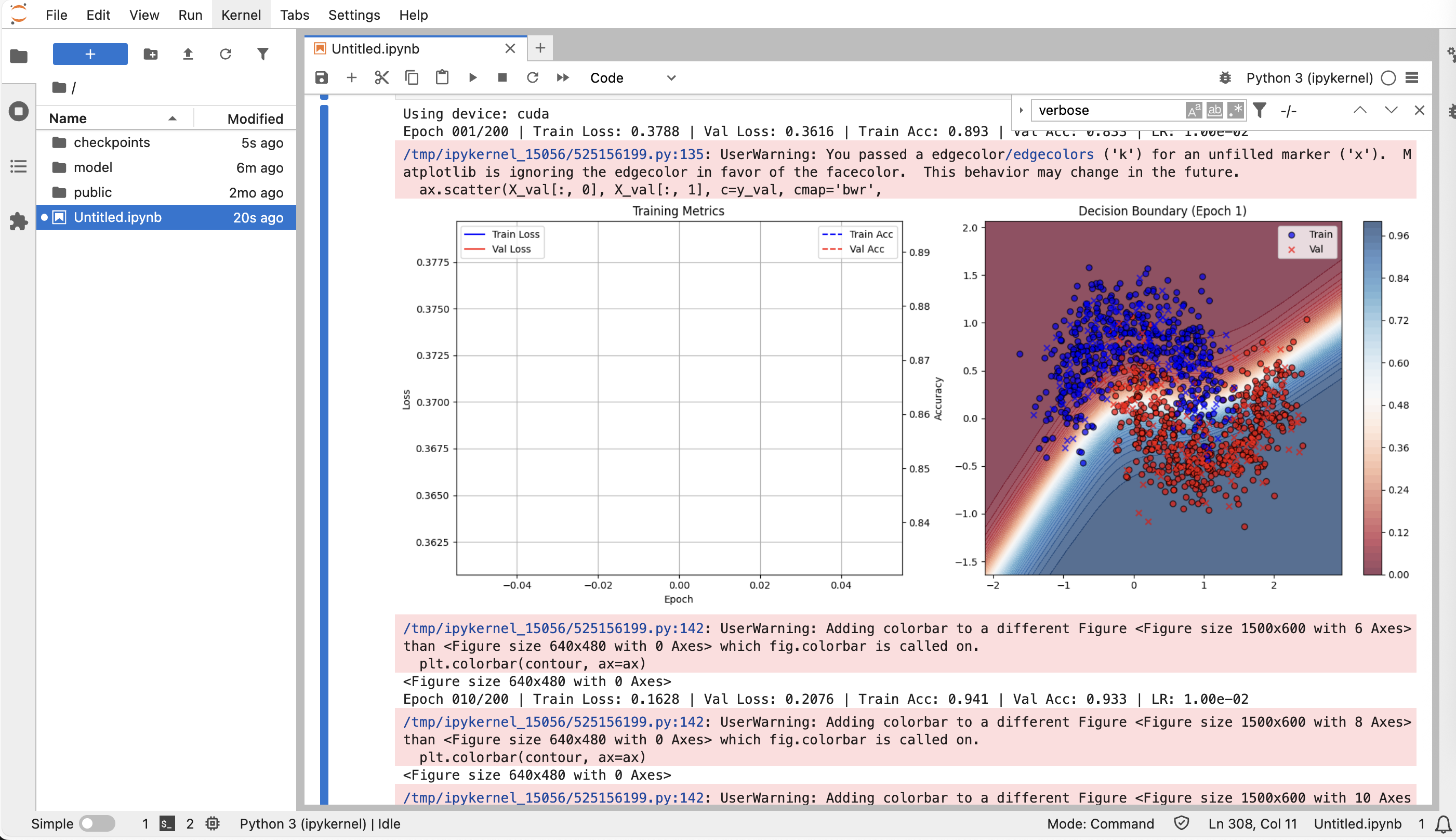
plt.show()

The following figure shows the output of the machine learning workflow.

Prerequisites​

Procedure​

Step 1: Create a Cloud Container Instance​

Step 2: Perform Machine Learning Tasks​

Prerequisites

Procedure

Step 1: Create a Cloud Container Instance

Step 2: Perform Machine Learning Tasks